-
Erik Strand authoredErik Strand authored

title: Final ProjectComputed Tomography
Background
- Radon Transform by Sigurdur Helgason
Introduction
Computed Tomography (CT) is used to turn 2d projections of a 3d shape like these (TODO insert image)
into a 3d model like this (TODO insert image).
This is pretty cool. In particular, voxels in the computed model can tell you the density at specific locations inside the scanned object, whereas pixels in the projections can only tell you the average density along lines that pass through the object. So we're getting a lot more out of those 2d images than meets the eye.
How does it work? That's what I'd like to understand. In particular, I hope to clearly explain the basic principles of CT, use them to implement a basic reconstruction from scratch, and experiment with existing solutions to get a sense of the state of the art.
I'm going to describe the algorithms in 2d, since it will make everything simpler. In this case we have an image like this (TODO insert image), and we'd like to reconstruct it only knowing its 1d projections at different angles.
Fourier Reconstruction
Fourier Slice Theorem
Let f : \mathbb{R}^2 \rightarrow \mathbb{R} be a density function. If we map density to brightness we can view f as describing an image. We'll assume that this function is defined everywhere, but is always zero outside some finite neighborhood of the origin (say, the bounds of the image).
The projection of f to the x axis is obtained by integrating along y:
p(x) = \int_\mathbb{R} f(x, y) dy
Meanwhile, the Fourier transform of f is
\hat{f}(u, v) = \int_\mathbb{R} \int_\mathbb{R} f(x, y) e^{-2 \pi i (u x + v y)} dx dy
Now comes the key insight. The slice along the u axis in frequency space is
\begin{align*} \hat{f}(u, 0) &= \int_\mathbb{R} \int_\mathbb{R} f(x, y) e^{-2 \pi i u x} dx dy \\ &= \int_\mathbb{R} \left( \int_\mathbb{R} f(x, y) dy \right) e^{-2 \pi i u x} dx \\ &= \int_\mathbb{R} p(x) e^{-2 \pi i u x} dx \\ &= \hat{p}(u) \end{align*}
So the Fourier transform of the 1d projection is a 1d slice through the 2d Fourier transform of the image. This result is known as the Fourier Slice Theorem, and is the foundation of most reconstruction techniques.
Since the x axis is arbitrary (we can rotate the image however we want), this works for other angles as well:
\hat{p}_\theta (\omega) = \hat{f} (\omega \cos \theta, \omega \sin \theta)
where p_\theta (r) is the projection of f onto the line that forms an angle \theta with the x axis. In other words, the Fourier transform of the 1D x-ray projection at angle \theta is the slice through the 2D Fourier transform of the image at angle \theta.
Conceptually this tells us everything we need to know about the reconstruction. First we take the 1D Fourier transform of each projection. Then we combine them by arranging them radially. Finally we take the inverse Fourier transform of the resulting 2d function. We'll end up with the reconstructed image.
It also tells us how to generate the projections, given that we don't have a 1d x-ray machine. First we take the Fourier transform of the image. Then we extract radial slices from it. Finally we take the inverse Fourier transform of each slice. These are the projections. This will come in handy for generating testing data.
Discretization
Naturally the clean math of the theory has be modified a bit to make room for reality. In particular, we only have discrete samples of f (i.e. pixel values) rather than the full continuous function (which in our current formalism may contain infinite information). This has two important implications.
First, we'll want our Fourier transforms to be discrete Fourier transforms (DFTs). Luckily the continuous and discrete Fourier transforms are effectively interchangeable, as long as the functions we work with are mostly spatially and bandwidth limited, and we take an appropriate number of appropriately spaced samples. You can read more about these requirements here.
Second, since we combine the DFTs of the projections radially, we'll end up with samples (of the 2D Fourier transform of our image) on a polar grid rather than a cartesian one. So we'll have to interpolate. This step is tricky and tends to introduce a lot of error. , but there are better algorithms out there that come closer to the theoretically ideal sinc interpolation. The popular gridrec method is one.
Implementation
I used FFTW to compute Fourier transforms. It's written in C and is very fast. I implemented my own polar resampling routine. It uses a Catmull-Rom interpolation kernel.
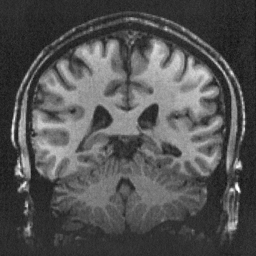
I started with this image of a brain from Wikimedia Commons.
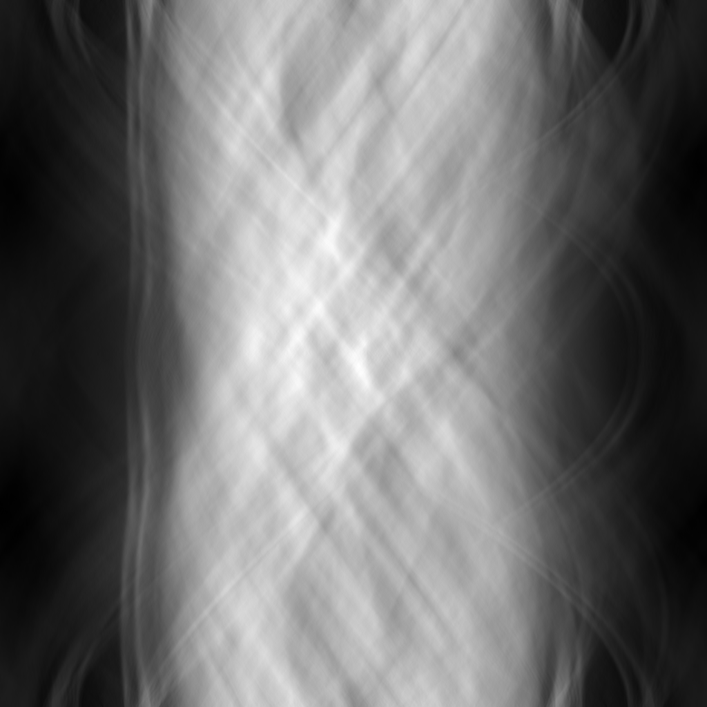
Fourier reconstruction produces a nice sinogram. Each row is one projection, with angle going from 0 at the top to \pi at the bottom, and r = 0 down the middle column. You can clearly see the skull (a roughly circular feature) unwrapped to a line on the left side of the sinogram.
The reconstruction, however, isn't so clean.

The Fourier library I'm using is solid (and indeed it reproduces images very well even after repeated applications), so the error must be coming from my interpolation code. Indeed, the high frequency content looks ok, but there's a lot of error in low frequency content. This is encoded in the middle of the Fourier transform, which is what is most distorted by the polar resampling. I could implement a resampling routine specifically designed for polar resampling, or indeed specifically for polar resampling for CT reconstruction, but there are better algorithms out there anyway so I'll move on.
Filtered Back Projection
It would be nice if we could avoid the interpolation required for Fourier reconstruction. The simplest way of doing so, and still the most popular method of performing image reconstruction, is called filtered back projection.
Theory
Let's hop back to the continuous theory for a moment. The Fourier reconstruction technique is based on the fact that f can be represented in terms of its projections p_\theta in polar coordinates.
\begin{align*} f(x, y) &= \int_\mathbb{R} \int_\mathbb{R} \hat{f}(u, v) e^{2 \pi i (ux + vy)} \mathrm{d}u \mathrm{d}v \\ &= \int_0^\pi \int_\mathbb{R} \hat{f}(\omega \cos \theta, \omega \sin \theta) e^{2 \pi i \omega (x \cos \theta + y \sin \theta)} \vert \omega \vert \mathrm{d} \omega \mathrm{d} \theta \\ &= \int_0^\pi \int_\mathbb{R} \hat{p}_\theta(\omega) e^{2 \pi i \omega (x \cos \theta + y \sin \theta)} \vert \omega \vert \mathrm{d} \omega \mathrm{d} \theta \\ \end{align*}
Instead of using interpolation to transform the problem back to cartesian coordinates where we can apply the usual (inverse) DFT, we can directly evaluate the above integral.
To simplify things a bit, note that the integral over \omega is itself a one dimensional inverse Fourier transform. In particular if we define
q_\theta(\omega) = \hat{p}_\theta(\omega) \vert \omega \vert
then the inner integral is just
\mathcal{F}^{-1}[q_\theta](x \cos \theta + y \sin \theta)
So overall
f(x, y) = \int_0^\pi \mathcal{F}^{-1}[q_\theta](x \cos \theta + y \sin \theta) \mathrm{d} \theta
Discretization
We'll replace the continuous Fourier transforms with DFTs as before.
The only remaining integral (i.e. that's not stuffed inside a Fourier transform) is over \theta, so most quadrature techniques will want samples of the integrand that are evenly spaced in \theta. We want the pixels in our resulting image to lie on a cartesian grid, so our integrand samples should be evenly spaced in x and y as well.
How do we compute \mathcal{F}^{-1}[q_\theta]? We are given samples of p_\theta(r) on a polar grid. Using the DFT, we can get samples of \hat{p}_\theta(\omega). They will be for the same \theta values, and evenly spaced frequency values \omega. So if we just multiply by \vert \omega \vert, we get the corresponding samples of q_\theta(\omega). Finally we just take the inverse DFT and we have samples of \mathcal{F}^{-1}[q_\theta] on a polar grid -- namely at the same (r, \theta) points we started out with.
This works out perfectly for \theta: we can take the samples we naturally end up with and use them directly for quadrature. For r, on the other hand, the regular samples we end up with won't line up with the values x \cos \theta + y \sin \theta that we want. So we'll still have to do some interpolation. But now it's a simple 1D interpolation problem that's much easier to do without introducing as much error. In particular, we only have to do interpolation in the spatial domain, so errors will only accumulate locally. Lanczos resampling would probably be the best, but I'll just use Catmull-Rom again since I already have it implemented.